Dual fisheye, 360° rig, and a lens pointing the wrong way

Research log · Hyuga.ai · Article 2

---

In the first article we talked about the gap between the perfect demos and what happens when you try to digitize a space yourself. This week we ran the full pipeline across three different datasets, timed every stage, and a few learnings came out that we didn’t see coming. The strangest one: the piece that fixed one of our reconstructions was the lens pointing toward what we didn’t care about seeing.

---

Before the photos: picking the right frames

The whole pipeline starts with a video of the scene that you then have to turn into images for COLMAP. The most obvious approach is to pull a frame every so many seconds. The problem is that if whoever is filming moves fast at some point, two consecutive frames can end up far apart in space, and COLMAP needs overlap between images to find points in common. At the same time, if the camera barely moves during a stretch, you end up with dozens of nearly identical frames that add no new information but do add processing time.

What we did was split the video into equal time segments and keep the best frame from each segment.

The process goes like this:

1. Extract every frame at a high fps (between 20 and 60 depending on the video).
2. Divide those frames into 200 equal-duration time segments.
3. For each segment, compute a sharpness score for every frame (we use the variance of the Laplacian, a fast way to measure how much detail an image has) and keep the sharpest one.
4. Delete everything else.
5. The result is 200 images with uniform temporal coverage, no gaps or clusters, where each one is the sharpest frame from its time window.

The sharpness difference between datasets was large. The azcuenaga one, filmed with good light and slow movement, had an average score of 518. The fuente-360 one, with more movement and worse light, came in at 124. That difference translates into how many features COLMAP detects per image and, therefore, into the density of the point cloud.

Segmenting and picking by sharpness is more setup work than extracting at a fixed interval, but it guarantees that every position along the path is represented by the best available frame.

---

The two-camera rig: how it actually works

Everything that follows in this article assumes a 360° camera with two fisheye lenses. The process also works with conventional cameras, individual fisheye lenses, or multi-camera setups. In the first article we explained why we chose 360°, basically the best balance between hardware cost and tolerance for capture error. Here we focus on that format because it’s where we’ve concentrated most of our research. If you work with a different configuration, some of these learnings apply just the same and others don’t.

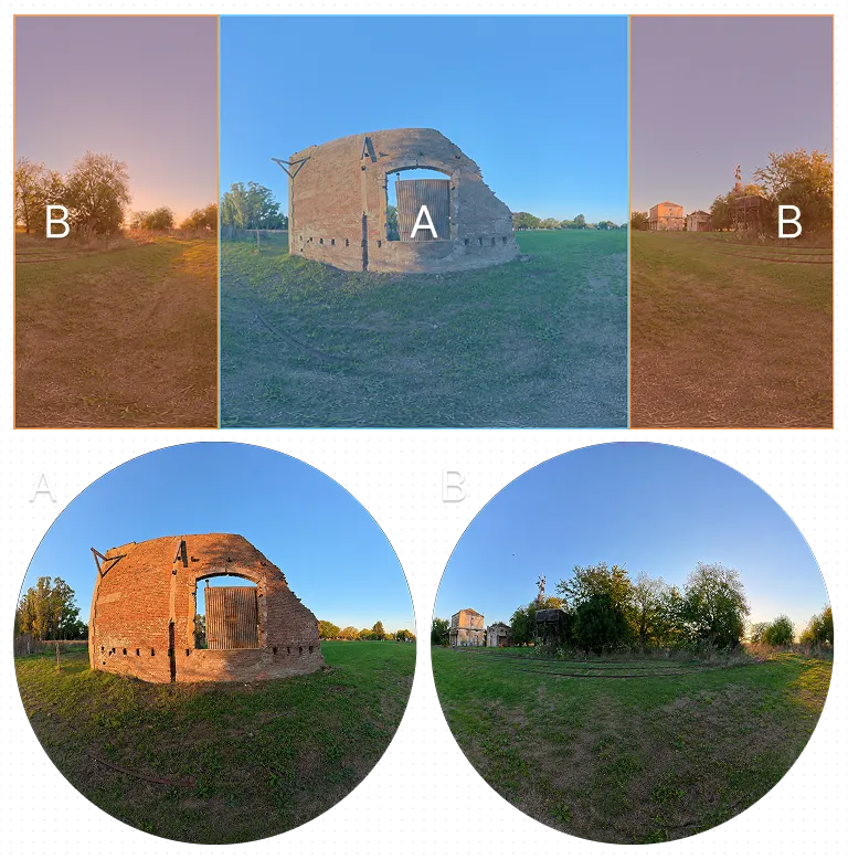
A 360° camera has two fisheye lenses, one pointing forward and one pointing backward, 180° apart. Each one captures a hemisphere. The video the camera records is an equirectangular image: the projection of the spherical world flattened into a rectangle, like a world map.

To feed COLMAP you have to do the reverse: take that equirectangular image and generate two separate fisheye images, one per hemisphere, matching what each lens would capture natively.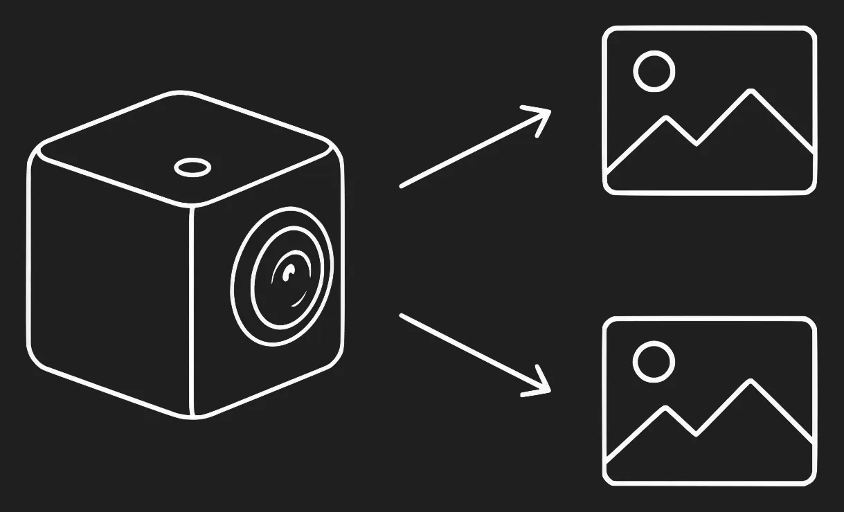

That sounds straightforward, but it was the first place where we made a mistake that cost us time.

The split that didn’t work

The first script we wrote used an OpenCV function (fisheye.undistortPoints) with a horizontal shift to separate the two cameras. It produced two images, but the geometry was wrong, it didn’t match how COLMAP models a rig. The images looked reasonable and the reconstruction still failed or came out unstable.

We ended up throwing that script away and rewriting it following COLMAP’s official flow (panorama_sfm.py). The change was to work with rays instead of pixels: for each pixel of the equirectangular image you compute the direction of the ray in 3D space, that ray gets rotated (cam0 to yaw 0°, cam1 to yaw 180°) and projected onto the corresponding fisheye model. It also generates a mask that assigns each pixel to exactly one camera, with no overlaps.

That process produces images COLMAP can use with the correct geometry, because the relationship between the two cameras is mathematically consistent with how it’s going to model the rig.

The angle matters: 64° vs 89°

With the split done right, the second problem showed up: how much angle to cover.

COLMAP’s fisheye example uses focal = height × 0.45, which at 3840px resolution gives a focal of 1728px. Each camera captures a cone of ~64° from the optical axis. Across 180° per hemisphere, that leaves a gap of ~26° with no coverage around the seam between the two cameras, on the sides (yaw ±90°).

In practice the gap is visible: areas with no points, weak matches right where the two cameras should connect.

We calculated the exact focal so the edge of the fisheye circle reaches 90° from the optical axis, the point where one hemisphere ends and the other begins. We call it full-seam. The resulting focal is 1234.3px (ratio 0.321 over the height), with a measured rim of 89.1°. The total point count between both configurations is similar, but the reprojection error drops and the seam closes. In a space meant to be explored freely, that uncovered area would have been visible in the final result.

COLMAP default (~64°) Full-seam (89°)

Using COLMAP’s default example leaves areas with no coverage at the seam. You have to compute the focal so the two hemispheres meet.

---

Rig vs single camera: what we found in this case

This week we also tested with a single perspective camera, on a dataset of a fountain in a plaza. Worth clarifying that this was a case where the single camera made sense: the fountain was fully visible within the frame of a single lens, no 360° needed. It was a legitimate test where a conventional camera could have worked. In our case, it didn’t.

The fisheye rig registered 400 images on the first try, with no calibration problems. The single camera needed four attempts to produce something usable, in large part because of calibration errors that don’t show up with the rig since the focal is computed from the geometry of the split.

Metric	Fisheye rig	Single camera
Images registered	400/400	200/200
Attempts needed	1	4
3D points	225k–319k	76k–89k
Average track length	16.8	~5–8
Calibration problems	None	Mis-scaled focal, wrong model

There are a few structural reasons that explain why the rig behaved better in this experiment.

With the rig, the focal comes from the geometry of the split: it’s an exact number COLMAP receives without having to estimate it. With the single camera and no reliable EXIF data, COLMAP needs an external prior. If that prior is mis-scaled, as in our case where the calibration had been done at a quarter of the real resolution, the process fails.

The rig also gives COLMAP a constraint the single camera doesn’t have: the relative position between the two lenses is fixed and known (one at 0°, the other at 180°). The mapper doesn’t have to solve that relationship from the feature matches; it already knows it. That reduces the degrees of freedom in the problem.

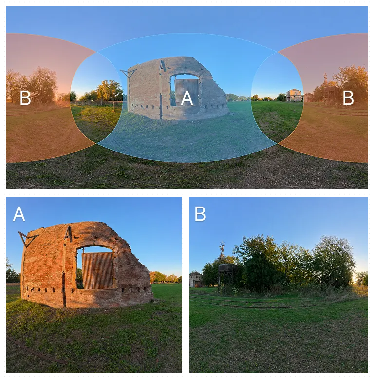
And then there’s the rear lens. If what you want to show is in front, that lens captures wall, ceiling, things that won’t appear in the final result. But COLMAP reconstructs the whole space and the camera’s position within it. More distinctive points around, in any direction, give the algorithm more anchors to figure out where the camera was at each shot. The two lenses together cover the whole sphere, so each point in the scene is seen from many angles. The average track length on the rig was 16.8 images per point; on the single camera, between 5 and 8. For scenes where a single camera has good calibration and good coverage, the results can get close. In our case they didn’t.

---

COLMAP: reconstruction modes and results from our tests

COLMAP has several independent variables that affect the result: the mapper can be incremental or global (GLOMAP), each stage can run on CPU or CUDA, and SIFT has a CPU and a GPU version. Changing any of those options shifts time, cloud density, and stability.

What follows are results from our tests on the azcuenaga dataset (fisheye rig, full-seam), with different combinations.

Test	Hardware	Mapper	Time	3D points
Incremental, local Mac	Apple M4 Pro, CPU	incremental	26.5 min	319,359
Incremental, pod	NVIDIA A6000, CUDA	incremental	~24 min	261,378
Global, pod	NVIDIA A6000, CUDA	global (GLOMAP)	15 min	226,018

With the incremental mapper, Mac CPU and pod CUDA took about the same time (24–26 min) but the Mac generated more points. The global run on the pod took half the time but produced ~30% fewer points than the incremental on the Mac.

Something we didn’t expect: in our tests, SIFT on GPU detected roughly 22% fewer points per image than on CPU, which translated into ~18% fewer 3D points at the end. If you run on a pod and the cloud comes out less dense than expected, that’s probably it.

To iterate quickly on the pipeline, global on GPU is more practical. For the densest cloud, incremental on Mac CPU gave the best time/quality balance.

The configuration we used

• Dual fisheye full-seam split. This is the configuration that closed the seam between hemispheres and gave the best results. COLMAP’s 0.45 preset leaves a gap at yaw ±90° that shows up in the final result.

• Preprocess the input before running COLMAP. From the 200 equirectangular panos (2:1 ratio), generate 400 fisheye images, 2 per pano, organized into two folders: pano_camera0/ (yaw 0°) and pano_camera1/ (yaw 180°).

• Focal computed for rim ≈ 90°, OPENCV_FISHEYE model, camera_mode PER_FOLDER. Don’t use the 0.45 preset. camera_mode PER_FOLDER tells COLMAP there’s one camera model per folder with equal intrinsics within each one, which is exactly the rig’s structure.

• Complete masks for both cameras. masks/pano_camera0/ and masks/pano_camera1/, with naming seg_001.jpg → seg_001.jpg.png. Without masks, the pixels shared between hemispheres break the rig.

---

What’s next

The questions we’re left with:

• How much does the density of COLMAP’s sparse cloud affect the final splat, versus other training parameters?
• Which parts of the full-seam pipeline (split, masks, etc.) can be automated without reintroducing geometry errors?
• In what kinds of scene does the dual fisheye rig keep beating a well-calibrated single camera, and in which ones does it stop mattering?

---

Hyuga.ai · research in progress Working with 360° or conventional cameras? We’d love to compare notes.